Data analysis
Flight curve and abundance index
The BMS methodology has been designed to provide estimates of numerical changes in butterfly populations. With this aim, at the end of each season, an annual index of abundance is calculated for each species and recording site, which includes estimated values for missing weeks.
The estimation of missing counts is achieved with maximum reliability by modelling the species flight curve with the regional GAM method (Schmucki et al., 2016). This method consists of adjusting for each season a general additive model to the weekly counts of a species using data from all itineraries that belong to a specific climatic region. In this way, a unique phenological curve is calculated for each region and season that, adapted to the abundance of the species in each locality, allows the counts of missing weeks to be estimated.
The sum of both real and estimated counts provides the annual abundance index of a species in a locality. These calculations are performed with the statistical package rbms (Schmucki et al., 2021).
Climatic regions
Both phenology and population dynamics of butterflies are strongly influenced by climate. For this reason, data are analysed separately and different phenological curves are generated, with a GAM model, for the three main climatic regions of the study area.
The climatic region to which an itinerary belongs has been established according to a thermal threshold, specifically, the number of annual hours in which a temperature of 21oC is exceeded (21DDG; according to data provided by the Meteorological Service of Catalonia).
Three climatic regions have been differentiated based on the following thresholds: alpine and subalpine region (≤ 0-150 DDG), humid Mediterranean region (150-400 DDG), arid Mediterranean region (≥ 400 DDG). These regions closely correspond to the bioclimatic regions defined by Metzguer et al. (2013), widely used in ecological modelling studies. As discussed above, populations of a species are considered to have the same flight curve across the set of CBMS stations in a given climatic region.
CBMS network map, showing the monitoring stations up to 2024 and the three climate regions to which they belong according to the climate model of Metzguer et al. (2013).
Flight curves
Data from transects where a species is considered to maintain populations are used to estimate the regional flight curve of that species each season. A species is considered to maintain a population in a locality when at least two individuals appear in a sampling year; otherwise, the species is considered to be occasional. In addition, the flight curve in a climate region is only calculated when data are available from a minimum of five transects with populations in at least one of the sampling years.
Although the flight curves of a species by region are estimated annually, on the web an average flight curve per species and region is shown that summarizes the observed phenological pattern for the set of available years.
The flight curve of the green-veined white (Pieris napi) has been estimated for two climatic regions, the alpine and the humid Mediterranean. The phenology is different in these two regions. While in the humid Mediterranean region the flight curve has three distinct peaks and maximum abundance in June, in the Alpine region the flight curve is delayed, has only two peaks and a maximum abundance in August–September. The interpretation of phenological curves can be complex since a peak does not always correspond simply to a generation. For example, in this figure the June–July peak in the humid Mediterranean region could in some years correspond to two widely overlapping generations.
Population trends
Local trends
Abundance indices are obtained for each transect and species, which give the annual relative abundance of the species in that locality. These indices are based on the sum of the weekly counts on the itinerary. When the regional flight curve of the species has been estimated using the GAM model, the annual index includes the actual counts and those estimated for the weeks lost. Otherwise, they only include actual counts. On the other hand, if the actual data corresponds to a very low percentage (less than 10%) of the 30 possible weeks, the model is not considered reliable enough to calculate an abundance index (in this case, the species appears as not evaluated).
On the web, in the species by transect sheets, annual indices for a species are standardized to a fixed distance of 100 m to facilitate comparison between populations and between species. The abundance indices that appear in the tables of both species and transect sheets correspond to the averages of all available years.
In the CBMS, a single annual abundance index is calculated per species, which reflects the success of the species over the entire flight period within the official 30-week season. If the phenology is clear enough to detect discrete generations, annual abundance indices can be calculated separately for each generation. However, given the complexity of the phenologies in the different climates in Catalonia, this option is discarded for current calculations. In addition, there is some variability depending on the year’s weather conditions, and bivoltine species with a partial third generation are common, as well as multivoltine species with a variable number of generations. In other BMS projects, such as the UKBMS in the UK, annual indices are distinguished by generations, and in bivoltine species only the second generation index is used, which is generally more abundant.
Local abundance indices are used to calculate local species trends along different transects. These trends are estimated from a linear regression between the logarithm of the local index (log [IA + 1]) and the year –– provided that the time series has eight or more years during which the species has appeared at least four years in a row. Otherwise, the species appears as ‘Not evaluated’. Local trends are classified into the following categories, according to the slope of the regression line and the level of significance:
- Strong regression: significant decline with more than 20% change over a 20-year period.
- Moderate regression: significant decline with less than 20% change over a 20-year period.
- Moderate increase: significant increase with less than 20% change over a 20-year period.
- Strong increase: significant increase with more than 20% change over a 20-year period.
- Stable: non-significant trend with small confidence intervals suggesting that there will be less than 20% change over a 20-year period.
- Uncertain: non-significant trend and confidence intervals large enough to consider that the trend could drive a change greater than 20% over a 20-year period.
- Extinct: when a local extinction phenomenon has been recorded without further recolonization. The criterion used to define an extinction is a sequence of four consecutive years without the appearance of a species in a locality, preceded by a sequence of at least four years with the presence of that species in the same place.
When a transect has been inactive for a long time, the trend graphs refer to the sampling period available for that station, without indicating what state the species is currently in.
Population trends of two species of Satyridae at the station El Cortalet, Natural Park of Aiguamolls de l'Empordà. The Gatekeeper, Pyronia tithonus, suffered a sharp decline in the second half of the 2000s, which eventually led to the extinction of the local population. By contrast, the Great Banded Grayling, Brintesia circe, colonized the area in 2004, and in the recent years has established a growing population. In both cases, trends appear to be a response to climatic factors, as the habitats where the two species occur have suffered little change at this site.
Regional trends
The BMS network provides data from a large number of stations and so a method is required to process all this information simultaneously. For this purpose, an annual regional index is calculated, which includes data from all the transects in each climate region and is used to calculate the trend of a species over time in that region. To estimate a regional index, a threshold of the presence of populations of the species in a minimum of five stations has been established, as used in the calculation of the flight curves.
To calculate the regional annual index of a species and its trend over time the statistical package rbms is used (Schmucki et al., 2021). To pool data from all transects where a species occurs into a single value, the annual regional index is estimated from a generalized linear model (GLM). This model corrects for the bias of transects that have more data than others by distributing the weight of the local data according to the percentage of the curve shown at each locality. At the same time, the model indirectly estimates the value that would correspond to the years in which the minimum of five transects for the calculation of the flight curve is not reached. Annual regional indices incorporate a 95% confidence interval, calculated using a bootstrap method that repeats calculations up to 500 times with random subsamples of data.
Regional population trends are shown only when a minimum of four consecutive years are available with data calculated or estimated according to the following criteria:
- The first year of a regional index series must be calculated with data from a minimum of five itineraries.
- Subsequent years must also exceed this minimum and there cannot be more than two consecutive years with insufficient data.
- When time series are interrupted for more than two years, the first year of the series becomes the one that guarantees that, from that point onwards, there are no discontinuities lasting more than two years.
- In the case of incomplete time series (in which data are missing from some years), population trends are calculated only when there are more calculated than estimated years.
Population trends are calculated separately for the three defined climatic regions (see Climatic regions section) but also for the set of all sampled stations.
Berger's clouded yellow (Colias alfacariensis) is currently in moderate regression across the CBMS network. However, at climatic region level a moderate regression is observed in the humid Mediterranean region but not in the Alpine region, where the trend (available for a shorter number of years) remains uncertain. Click the legend categories to enable/disable the series.
Habitat preferences and habitat indicators
The CBMS collects precise information on the abundance of species in different habitats as transects are divided into different sections according to the habitats sampled. These data make it possible to calculate several indices that detail the species' preferences for different environments, which then form the basis for the calculation of multi-specific habitat indicators.
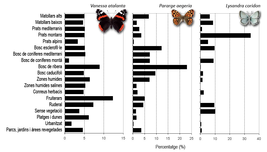
The figure shows three species with very different habitat preferences. The red admiral, Vanessa atalanta, is a generalist species that can be found in almost any type of environment due to its great dispersive capacity. The speckled wood, Pararge aegeria is a butterfly that appears mainly in forest-type habitats, where it is very common. On the other hand, the chalkhill blue Lysandra coridon, is a specialist species of montane meadows in the Pyrenees and pre-Pyrenees.
Habitat Specialization Index (SSI)
Counts correspond to sections dominated by different plant communities, which can be assigned to broad habitat types. This allows us to explore in which environments the populations of a given species reach their maximum densities. The characterization of the plant communities in the sections of the itineraries (which is done according to the CORINE classification), started in 2000 and is revised every six years for each itinerary. This information is essential for calculating habitat indicators and detecting problems that affect biodiversity in particular habitats and environments.
Read more...
The original plant communities classified according to CORINE have been grouped into 19 broader habitat categories that are useful for understanding butterfly preferences and ecology. These are:
- Tall shrubland
- Low shrubland
- Mediterranean meadows
- Montane meadows
- Alpine meadows
- Schlerophyllous forests
- Mediterranean coniferous forests
- Montane coniferous forests
- Riparian forests
- Deciduous forests
- Wetlands
- Saline wetlands
- Mountain wetlands
- Herbaceous crops
- Fruit trees
- Ruderal vegetation
- Bare ground
- Beaches and dunes
- Urbanized
- Urban parks, gardens and revegetated areas
A detailed description of each category can be found in the results by habitat section.
The preference of a species for a habitat is calculated from the density it presents in that habitat in the CBMS network as a whole compared to the densities of the remaining 19 habitats. For a graphical representation, densities for a habitat are shown as a percentage of the total sum of densities in the 20 defined habitats.
The calculations are as follows. First, for each species the average density (average annual number of individuals observed in 100 m of transect) is obtained in the different habitats of a specific itinerary. This density is calculated from the data per section, multiplying the average annual density in this section by the percentage of coverage of the habitats present. A minimum coverage threshold of 25% has been established for one type of habitat per stretch, thus eliminating from the analysis those habitats that are poorly represented and that probably do not explain the presence of a certain species in this section.
Secondly, all the itineraries where the species appears are taken into account when calculating its average density in each of the 20 habitats of the CBMS network. In this process, a density of zero is assigned to those habitats where the species in question has not been observed, so that finally the densities are expressed as a percentage for a fixed total of 20 habitats.
These values show the distribution of all individuals of a species detected in the CBMS among the 20 habitat categories. When a species has a strong preference for a particular habitat, most specimens are linked to that habitat, while the percentages of occurrence in other habitats are very low. On the other hand, the percentages of occurrences are more equally distributed among the different categories when a species is generalist. To quantify these preferences, the habitat specialization index (SSI) is calculated as the coefficient of variation (CV = standard deviation/mean) of the density distribution (expressed as a percentage) in the 20 habitats. The more specialized a species is, the more heterogeneous the density distribution and the higher the SSI. By contrast, generalist species have similar densities in many habitats and thus their SSI is low. In order to help visualize habitat specialization in species, these values have been scaled from 1 (most generalist) to 10 (most specialist).
Calculations of habitat preference and the SSI index have only been carried out for those species occurring in a minimum of five transects. Likewise, the data of a species in a certain type of habitat have not been taken into account for those habitats that appear in a single transect for the species in question. In this way, unrealistic associations between butterfly species and certain habitats are avoided. However, it should be noted that habitat preference values may still show biases due to the sample size of each species and particular butterfly behaviour not necessarily linked to a given habitat type (e.g. mud-puddling and hilltopping behaviour, etc.). Thus, data quality increases as transect time series become longer and as the number of stations available for a given species increases.
Closed - Open Index (TAO)
The TAO index places the set of the species in the CBMS along a gradient of preference from more closed to open habitats. The value given for each species corresponds to a range that runs from -1 (for species with a preference for closed habitats) to 1 (for species with a preference for open habitats) (Ubach et al., 2020).
Read more...
To calculate the TAO, first of all a binary classification of all plant communities represented in the network is made, according to whether they are open, to which the value of 1 is assigned, or closed, to which the value assigned is -1. Then, for each section, a final value is calculated by multiplying the coverage percentages of the plant communities present by the corresponding binary value (-1 or +1). Sections that have a positive resulting value are considered open, while those with a negative number are considered closed. To avoid the problem that sections with values very close to 0 are classified as open or closed even though they in fact consist of a mixture between the two situations, we apply a filter: only those sections in which the final value is ≥ | 0.1 | are considered. Therefore, sections with values in the range (-0.1, 0.1) are discarded.
Once all sections have been reclassified as open or closed, two averages of species density are calculated for each transect: one for the set of open sections (Dopen) and the other for closed sections (Dclosed). The TAO index is then calculated from these two averages according to the formula developed by Suggitt et al. (2012).
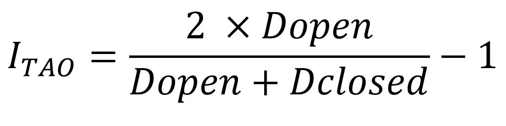
The final TAO index value for a species is the average of the TAO indices obtained in all the itineraries where a species occurs.
For the calculation of the index a species must be present in at least five transects (as for the SSI index and habitat preferences calculations).
Other habitat indicators
General abundance index
The general abundance index uses
all species from the study region for which sufficient data are
available to calculate a regional abundance index. The multispecies
index (MSI) is constructed from the geometric mean of the regional
abundance indices, including all species for which these indices are
available for at least two consecutive years. This process is repeated
500 times using bootstrap iterations, which also allow the calculation
of 95% confidence intervals. Finally, a smoothed trend is generated
using a loess fit (span = 0.75, degree = 2). MSI values are rescaled to
start at 100 in the first year, which facilitates comparisons and
interpretation. The trend and statistical significance of the MSI are
calculated by applying a linear regression to the smoothed indicator.
This calculation is performed using the software TRIM (Pannekoek &
van Strien 2005), which classifies the trend into several categories
based on the magnitude of temporal change and the associated confidence
intervals.
Abundance index for grasslands and forests
This index uses all species from the study region following a methodology similar to the one described above, but weighting each species according to its TAO index (see Habitat preferences and indicators). For the grassland indicator, the annual regional index of each species is multiplied by its corresponding TAO value (recalculated as TAO + 1 so that all values are positive within the 0–2 range). In this way, a species fully dependent on grasslands has a weight of 2, whereas a species fully dependent on forests has a weight of 0 (i.e. it does not contribute to the overall grassland indicator). For the forest indicator, a symmetrical weighting is applied: a strictly forest species receives a weighting value of 2, whereas a strictly grassland species receives a weighting value of 0.
Recommended references
- Julliard, R., Clavel, J., Devictor, V., Jiguet, F., Couvet, D. (2006) Spatial segregation of specialists and generalists in bird communities. Ecology Letters 9:1237–1244
- Melero, Y., Stefanescu, C., Pino, J. (2016) General declines in Mediterranean butterflies over the last two decades are modulated by species traits. Biological Conservation, 201: 336-342. DOI 10.1016/j.biocon.2016.07.029
- Metzger, M.J., Bunce, R.G.H., Jongman, R.H.G., Sayre,R., Trabucco, A., Zomer. R. (2013) A high-resolution bioclimate map of the world: a unifying framework for global biodiversity research and monitoring. Global Ecology and Biogeography, 22: 630-638.
- Schmucki, R., Pe'er, G., Roy, D.B., Stefanescu, C., Van Swaay, C.A.M., Oliver, T.H., Kuussaari, M., Van Strien, A., Ries, L., Settele, J., Musche, M., Carnicer, J., Schweiger, O., Brereton, T., Harpke, A., Heliölä, J., Kühn, E., Julliard, R (2016) Regionally informed abundance index for supporting integrative analyses across butterfly monitoring schemes. Journal of Applied Ecology, 53: 501-510. DOI 10.1111/1365-2664.12561
- SCHMUCKI R., HARROWER C.A., DENNIS E.B. (2021) rbms: Computing generalised abundance indices for butterfly monitoring count data. R package version 1.1.0. https://github.com/RetoSchmucki/rbms
- Stefanescu, C., Torre, I, Jubany, J., Páramo, F. (2011) Recent trends in butterfly populations from north-east Spain and Andorra in the light of habitat and climate change. Journal of Insect Conservation 15: 83-93. DOI 10.1007/s10841-010-9325-z
- Ubach, A., Páramo, F., Gutiérrez, C., Stefanescu, C. (2020) Vegetation encroachment drives changes in the composition of butterfly assemblages and species loss in Mediterranean ecosystems. Insect Conservation and Diversity, 13: 151-161. DOI 10.1111/icad.12397
Web map | Legal notes | Credits
Project in agreement with:


In collaboration with: